library(mesa)
#> Loading required package: qsea
#> Loading required package: dplyr
#>
#> Attaching package: 'dplyr'
#> The following objects are masked from 'package:stats':
#>
#>     filter, lag
#> The following objects are masked from 'package:base':
#>
#>     intersect, setdiff, setequal, union
#>
#> Attaching package: 'mesa'
#> The following object is masked from 'package:qsea':
#>
#>     getPCA
library(dplyr)
library(ggplot2)
library(tidyr)
library(stringr)
Generating tables of values from a qseaSet
qsea has several different types of values that can be
returned per window. You can get a table of raw counts per window with
getCountTable:
exampleTumourNormal %>%
    getCountTable()
#> Generating table of counts values for 819 regions across 10 samples.
#> # A tibble: 819 × 14
#>    seqnames    start      end CpG_density Colon1_N Colon1_T Colon2_N Colon2_T
#>    <fct>       <int>    <int>       <dbl>    <dbl>    <dbl>    <dbl>    <dbl>
#>  1 7        25002001 25002300        5.51        0        1        1        1
#>  2 7        25005001 25005300       13.4         1        0        0        0
#>  3 7        25008601 25008900        5.57        0        0        0        1
#>  4 7        25011301 25011600        5.10        0        1        0        1
#>  5 7        25017601 25017900        8.38        0        0       18       14
#>  6 7        25017901 25018200       17.9         0        4       11       18
#>  7 7        25018201 25018500       16.5         1        0        4        4
#>  8 7        25018501 25018800       17.5         0        0        1        0
#>  9 7        25018801 25019100       15.3         1        0        2        3
#> 10 7        25019101 25019400       18.2         3        2        9        4
#> # ℹ 809 more rows
#> # ℹ 6 more variables: Lung1_N <dbl>, Lung1_T <dbl>, Lung2_N <dbl>,
#> #   Lung2_T <dbl>, Lung3_N <dbl>, Lung3_T <dbl>
but this is not particularly useful, as different samples have
generally been sequenced to different read depths. Note that the
annotation of the qseaSet regions is included in this
output, notably the CpG_density that is described in
vignette("generation", package = "mesa").
The next option is normalised reads per million (NRPM). This normalises the number of reads by the depth of sequencing, as well as by copy number variation.
exampleTumourNormal %>%
    getNRPMTable()
#> Generating table of nrpm values for 819 regions across 10 samples.
#> Loading required namespace: GenomeInfoDb
#> # A tibble: 819 × 14
#>    seqnames    start      end CpG_density Colon1_N Colon1_T Colon2_N Colon2_T
#>    <fct>       <int>    <int>       <dbl>    <dbl>    <dbl>    <dbl>    <dbl>
#>  1 7        25002001 25002300        5.51    0        0.131    0.246    0.178
#>  2 7        25005001 25005300       13.4     0.263    0        0        0
#>  3 7        25008601 25008900        5.57    0        0        0        0.178
#>  4 7        25011301 25011600        5.10    0        0.131    0        0.178
#>  5 7        25017601 25017900        8.38    0        0        4.42     2.50
#>  6 7        25017901 25018200       17.9     0        0.523    2.70     3.21
#>  7 7        25018201 25018500       16.5     0.263    0        0.983    0.713
#>  8 7        25018501 25018800       17.5     0        0        0.246    0
#>  9 7        25018801 25019100       15.3     0.263    0        0.491    0.535
#> 10 7        25019101 25019400       18.2     0.788    0.262    2.21     0.713
#> # ℹ 809 more rows
#> # ℹ 6 more variables: Lung1_N <dbl>, Lung1_T <dbl>, Lung2_N <dbl>,
#> #   Lung2_T <dbl>, Lung3_N <dbl>, Lung3_T <dbl>
Finally, we can request beta values. Beta values are measures of
methylation, scaled to lie between 0 and 1, where 0 means that the
window is unmethylated and 1 is methylated. These are scaled with
respect to a number of further metrics, including the region’s
CpG_density, background noise and the sample enrichment
profile, and are therefore the most useful value to consider when
comparing methylation between samples.
exampleTumourNormal %>%
    getBetaTable()
#> Generating table of beta values for 819 regions across 10 samples.
#> # A tibble: 819 × 14
#>    seqnames    start      end CpG_density Colon1_N Colon1_T Colon2_N Colon2_T
#>    <fct>       <int>    <int>       <dbl>    <dbl>    <dbl>    <dbl>    <dbl>
#>  1 7        25002001 25002300        5.51  NA        0.347   NA        0.369
#>  2 7        25005001 25005300       13.4    0.0565   0.0171   0.0275   0.0165
#>  3 7        25008601 25008900        5.57  NA        0.204   NA        0.363
#>  4 7        25011301 25011600        5.10  NA        0.382   NA        0.406
#>  5 7        25017601 25017900        8.38   0.122    0.0695   0.918    0.818
#>  6 7        25017901 25018200       17.9    0.0240   0.0660   0.265    0.250
#>  7 7        25018201 25018500       16.5    0.0472   0.0143   0.112    0.0669
#>  8 7        25018501 25018800       17.5    0.0241   0.0140   0.0426   0.0133
#>  9 7        25018801 25019100       15.3    0.0493   0.0149   0.0692   0.0559
#> 10 7        25019101 25019400       18.2    0.0932   0.0380   0.220    0.0646
#> # ℹ 809 more rows
#> # ℹ 6 more variables: Lung1_N <dbl>, Lung1_T <dbl>, Lung2_N <dbl>,
#> #   Lung2_T <dbl>, Lung3_N <dbl>, Lung3_T <dbl>
Note that for some windows an NA value will be returned. This occurs
when fewer than three reads would be required for the window to be fully
methylated, at the read depth and enrichment profile calculated per
sample. These occur particularly at windows with a low
CpG_density.
All three of these functions take an option
useGroupMeans that determines whether to average over the
group column of the qseaSet sampleTable, which
can be useful when you have biological or technical replicates for
example.
In the example qseaSet, group is the same as
sample_name, so we need to change that to see the
effect:
exampleTumourNormal %>%
    getBetaTable(useGroupMeans = FALSE)
#> Generating table of beta values for 819 regions across 10 samples.
#> # A tibble: 819 × 14
#>    seqnames    start      end CpG_density Colon1_N Colon1_T Colon2_N Colon2_T
#>    <fct>       <int>    <int>       <dbl>    <dbl>    <dbl>    <dbl>    <dbl>
#>  1 7        25002001 25002300        5.51  NA        0.347   NA        0.369
#>  2 7        25005001 25005300       13.4    0.0565   0.0171   0.0275   0.0165
#>  3 7        25008601 25008900        5.57  NA        0.204   NA        0.363
#>  4 7        25011301 25011600        5.10  NA        0.382   NA        0.406
#>  5 7        25017601 25017900        8.38   0.122    0.0695   0.918    0.818
#>  6 7        25017901 25018200       17.9    0.0240   0.0660   0.265    0.250
#>  7 7        25018201 25018500       16.5    0.0472   0.0143   0.112    0.0669
#>  8 7        25018501 25018800       17.5    0.0241   0.0140   0.0426   0.0133
#>  9 7        25018801 25019100       15.3    0.0493   0.0149   0.0692   0.0559
#> 10 7        25019101 25019400       18.2    0.0932   0.0380   0.220    0.0646
#> # ℹ 809 more rows
#> # ℹ 6 more variables: Lung1_N <dbl>, Lung1_T <dbl>, Lung2_N <dbl>,
#> #   Lung2_T <dbl>, Lung3_N <dbl>, Lung3_T <dbl>

exampleTumourNormal %>%
    mutate(group = str_remove(sample_name,"\\d")) %>%
    getBetaTable(useGroupMeans = TRUE)
#> Generating table of beta values for 819 regions across 4 sample groups.
#> # A tibble: 819 × 8
#>    seqnames    start      end CpG_density  Colon_N Colon_T Lung_N Lung_T
#>    <fct>       <int>    <int>       <dbl>    <dbl>   <dbl>  <dbl>  <dbl>
#>  1 7        25002001 25002300        5.51 NaN       0.358  0.372  0.222
#>  2 7        25005001 25005300       13.4    0.0420  0.0168 0.0404 0.0748
#>  3 7        25008601 25008900        5.57 NaN       0.284  0.263  0.303
#>  4 7        25011301 25011600        5.10 NaN       0.394  0.373  0.416
#>  5 7        25017601 25017900        8.38   0.520   0.444  0.877  0.721
#>  6 7        25017901 25018200       17.9    0.145   0.158  0.180  0.123
#>  7 7        25018201 25018500       16.5    0.0797  0.0406 0.0588 0.0659
#>  8 7        25018501 25018800       17.5    0.0334  0.0137 0.0262 0.0293
#>  9 7        25018801 25019100       15.3    0.0592  0.0354 0.0940 0.113
#> 10 7        25019101 25019400       18.2    0.156   0.0513 0.0753 0.0693
#> # ℹ 809 more rows
Now the table has one column per group (four here) rather than one
per sample. Windows where no sample in a group has a beta value are
returned as NaN.
We explicitly note that qsea incorporates the uncertainty of the
measurements in its beta value estimations. This means that the values
returned as beta values are actually the median of this
estimate, with an associated confidence interval (which can be queried,
see qsea::makeTable). In practice, this means that samples
with high coverage can return values very close to 0 and 1, but the same
sample with less coverage might return 0.1 or 0.9. This can have an
effect on clustering and PCAs for example.
Quality Control
One extremely important aspect of any sequencing experiment is quality control (QC), and ME-seq is no exception. Alongside the typical QC steps on the bam files themselves (although a raised CG content should obviously be expected following enrichment), there are several methylation-specific steps to consider.
Relative Enrichment
The first metric used for QC is a relative enrichment metric, known
as relH. This was first introduced in the
MEDIPS package, via the MEDIPS.CpGenrich()
function, and is a metric to express the proportion of CG dinucleotides,
compared to the reference genome. The relative enrichment
relH is calculated in the following way:
- For each mapped DNA fragment, retrieve the end-to-end DNA spanned on the reference sequence. This is used instead of the reads themselves, as a fragment will often be longer than the read(s) sequenced at its ends, and may therefore contain CGs not covered by the reads.
- In these sequences, count how many CGs are present in total, and divide by the total number of base pairs covered.
- Divide by the same ratio, calculated for the entire genome.
This is therefore a measure of how many more CGs are present in the fragments covered within the bam file, compared to the reference genome.
Within mesa, this metric is calculated through
makeQset, as part of the information added to the
libraries table on the qseaSet. As a rough
guideline, for the T7-MBD-seq data studied by the package authors,
relH values of 4-5 were typical, with a minimum of 2.5-3
regarded as acceptable. Typical values may depend on enrichment method
and sample type.
We can use the addLibraryInformation function to add the
information in the libraries table directly onto the
sampleTable:
exampleTumourNormal %>%
    addLibraryInformation() %>%
    getSampleTable() %>%
    dplyr::select(sample_name, relH)
#>          sample_name     relH
#> Colon1_N    Colon1_N 5.567633
#> Colon1_T    Colon1_T 4.921130
#> Colon2_N    Colon2_N 5.399262
#> Colon2_T    Colon2_T 5.686246
#> Lung1_N      Lung1_N 4.463002
#> Lung1_T      Lung1_T 4.406991
#> Lung2_N      Lung2_N 4.602440
#> Lung2_T      Lung2_T 4.753918
#> Lung3_N      Lung3_N 5.111422
#> Lung3_T      Lung3_T 5.078306
When a non-enriched (“Input”) sample is used to calculate copy number
variation, an equivalent calculation is also performed on these
non-enriched fragments. This is also stored in the
libraries table, in columns starting with
input_:
exampleTumourNormal %>%
    addLibraryInformation() %>%
    getSampleTable() %>%
    dplyr::select(sample_name, input_relH)
#>          sample_name input_relH
#> Colon1_N    Colon1_N   1.506917
#> Colon1_T    Colon1_T   1.446767
#> Colon2_N    Colon2_N   1.608130
#> Colon2_T    Colon2_T   1.474401
#> Lung1_N      Lung1_N   1.437550
#> Lung1_T      Lung1_T   1.481526
#> Lung2_N      Lung2_N   1.418541
#> Lung2_T      Lung2_T   1.400016
#> Lung3_N      Lung3_N   1.644814
#> Lung3_T      Lung3_T   1.623274
Values of input_relH between 1.3 and 1.6 were observed
in non-enriched data studied by the package authors. These values above
1 indicate that more CGs are seen in the sequenced fragments than would
be expected from the genomic sequence. This is possibly due to the
evolutionary suppression of CG dinucleotides outside of
specific contexts, meaning they are less common in those areas of the
genome that are repetitive and hence less easy to map. This is likely to
depend on the particular sequencing methods and the sample type under
consideration.
We expect to see an increase in the enrichment metric between the enriched and non-enriched data:
exampleTumourNormal %>%
    addLibraryInformation() %>%
    getSampleTable() %>%
    dplyr::select(sample_name, relH_MeCap = relH, relH_Input = input_relH) %>%
    pivot_longer(matches("relH"),
                names_prefix = "relH_",
                names_to = "enrichment",
                values_to = "relH") %>%
    ggplot(aes(x = sample_name, y = relH, col = enrichment)) +
    geom_point() +
    theme_bw() +
    theme(axis.text.x = element_text(angle = 45, hjust = 1))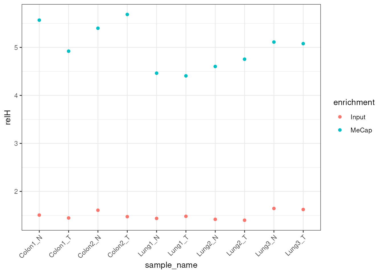
There is a second relative enrichment metric defined by the
MEDIPS package, known as GoGe, that is also
calculated globally in a similar way but considers the ratio between the
number of CGs present in the fragments compared to the
number of Cs and Gs independently. This is
calculated and stored in the libraries information
alongside the relH metric.
Fragments without pattern
The libraries table also records how many fragments do
not contain a CG at all. This can be a measure of background noise.
Hyper-stably methylated regions
Another metric used for quality control is based on windows that are
known to be commonly methylated across a range of tissues and diseases.
For instance, for the human genome, Edgar et al. (2014)
identified probes from the Illumina 450k methylation array that were
consistently methylated in over 1700 samples. We take windows covered by
these probes, calculate beta values for them, and then determine the
proportion of these windows that have a beta value above a threshold of
0.8; we call this metric hyperStableEdgar. Samples with
lower enrichment scores (relH) require a greater coverage
depth for beta values to reach a given threshold. The metric therefore
incorporates both the coverage depth and how well the enrichment has
worked.
As noted above, windows with low CpG_density are more
likely to have an NA beta value. To avoid considering windows that
typically have a missing beta value across most samples, the calculation
of hyperStableEdgar is restricted to windows that have a
CpG_density of at least 5. Samples with insufficient
coverage and/or enrichment will still have missing beta values for some
windows with CpG_density above this minimum value. These
missing beta values are treated as zero when calculating
hyperStableEdgar.
For hg38, these hyper-stable methylated probes are provided in a data
object, hg38UltraStableProbes, and the function
addHyperStableFraction calculates the
hyperStableEdgar metric and adds it as a column to the
sampleTable. Note that the function will not work with the provided
example data, as there is no overlap of the probes with the windows in
the example dataset (i.e.
filterByOverlaps(exampleTumourNormal, hg38UltraStableProbes)
has no windows).
For the T7-MBD-seq data studied by the package authors, a
hyperStableEdgar value of at least 0.4 was considered
acceptable. Again, suitable values may depend on enrichment method and
sample type.
Summary
In the package authors’ experience, the three metrics
valid_fragments, relH and
hyperStableEdgar are the most useful for quality control.
For 300 bp windows on the human genome with T7-MBD-seq data, the authors
considered a relH of at least 2.5–3, a
hyperStableEdgar value of at least 0.4 (40%), and around
3,000,000 valid_fragments acceptable. Samples that met the
relH and hyperStableEdgar thresholds usually
also met the valid_fragments threshold. These values are
provided as guidelines rather than strict thresholds; suitable values
will depend on the enrichment protocol (MBD-seq or MeDIP-seq), the
sample type and the sequencing depth, so we recommend choosing
thresholds from the distribution of these metrics in your own data.
Session info
#> R version 4.6.1 (2026-06-24)
#> Platform: x86_64-pc-linux-gnu
#> Running under: Ubuntu 24.04.4 LTS
#>
#> Matrix products: default
#> BLAS:   /usr/lib/x86_64-linux-gnu/openblas-pthread/libblas.so.3
#> LAPACK: /usr/lib/x86_64-linux-gnu/openblas-pthread/libopenblasp-r0.3.26.so;  LAPACK version 3.12.0
#>
#> locale:
#>  [1] LC_CTYPE=en_US.UTF-8       LC_NUMERIC=C
#>  [3] LC_TIME=en_US.UTF-8        LC_COLLATE=en_US.UTF-8
#>  [5] LC_MONETARY=en_US.UTF-8    LC_MESSAGES=en_US.UTF-8
#>  [7] LC_PAPER=en_US.UTF-8       LC_NAME=C
#>  [9] LC_ADDRESS=C               LC_TELEPHONE=C
#> [11] LC_MEASUREMENT=en_US.UTF-8 LC_IDENTIFICATION=C
#>
#> time zone: UTC
#> tzcode source: system (glibc)
#>
#> attached base packages:
#> [1] stats     graphics  grDevices utils     datasets  methods   base
#>
#> other attached packages:
#> [1] stringr_1.6.0    tidyr_1.3.2      ggplot2_4.0.3    mesa_0.99.8.9000
#> [5] dplyr_1.2.1      qsea_1.38.0
#>
#> loaded via a namespace (and not attached):
#>  [1] tidyselect_1.2.1            farver_2.1.2
#>  [3] Biostrings_2.80.2           S7_0.2.2
#>  [5] bitops_1.1-0                fastmap_1.2.0
#>  [7] RCurl_1.98-1.20             GenomicAlignments_1.48.0
#>  [9] XML_3.99-0.25               digest_0.6.39
#> [11] lifecycle_1.0.5             statmod_1.5.2
#> [13] magrittr_2.0.5              compiler_4.6.1
#> [15] rlang_1.3.0                 sass_0.4.10
#> [17] tools_4.6.1                 utf8_1.2.6
#> [19] yaml_2.3.12                 data.table_1.18.6.1
#> [21] rtracklayer_1.72.0          knitr_1.52
#> [23] labeling_0.4.3              S4Arrays_1.12.1
#> [25] htmlwidgets_1.6.4           curl_8.1.0
#> [27] DelayedArray_0.38.2         RColorBrewer_1.1-3
#> [29] abind_1.4-8                 BiocParallel_1.46.0
#> [31] HMMcopy_1.54.0              withr_3.0.3
#> [33] purrr_1.2.2                 BiocGenerics_0.58.1
#> [35] desc_1.4.3                  grid_4.6.1
#> [37] stats4_4.6.1                scales_1.4.0
#> [39] gtools_3.9.5                SummarizedExperiment_1.42.0
#> [41] cli_3.6.6                   rmarkdown_2.32
#> [43] crayon_1.5.3                ragg_1.5.2
#> [45] generics_0.1.4              otel_0.2.0
#> [47] httr_1.4.9                  rjson_0.2.23
#> [49] cachem_1.1.0                parallel_4.6.1
#> [51] XVector_0.52.0              restfulr_0.0.17
#> [53] matrixStats_1.5.0           vctrs_0.7.3
#> [55] Matrix_1.7-6                jsonlite_2.0.0
#> [57] IRanges_2.46.0              S4Vectors_0.50.3
#> [59] systemfonts_1.3.2           limma_3.68.5
#> [61] jquerylib_0.1.4             glue_1.8.1
#> [63] pkgdown_2.2.1               codetools_0.2-20
#> [65] stringi_1.8.9               gtable_0.3.6
#> [67] GenomeInfoDb_1.48.0         UCSC.utils_1.8.0
#> [69] BiocIO_1.22.0               GenomicRanges_1.64.0
#> [71] tibble_3.3.1                pillar_1.11.1
#> [73] htmltools_0.5.9             Seqinfo_1.2.0
#> [75] BSgenome_1.80.0             R6_2.6.1
#> [77] textshaping_1.0.5           evaluate_1.0.5
#> [79] lattice_0.23-1              Biobase_2.72.0
#> [81] Rsamtools_2.28.0            cigarillo_1.2.1
#> [83] memoise_2.0.1               bslib_0.12.0
#> [85] SparseArray_1.12.3          xfun_0.61
#> [87] fs_2.1.0                    MatrixGenerics_1.24.0
#> [89] zoo_1.9-1                   pkgconfig_2.0.3