library(mesa)
#> Loading required package: qsea
#> Loading required package: dplyr
#>
#> Attaching package: 'dplyr'
#> The following objects are masked from 'package:stats':
#>
#>     filter, lag
#> The following objects are masked from 'package:base':
#>
#>     intersect, setdiff, setequal, union
#>
#> Attaching package: 'mesa'
#> The following object is masked from 'package:qsea':
#>
#>     getPCA
Introduction
This vignette introduces the mesa package, which is
designed to help analyse methylation enrichment sequencing data.
Methylation enrichment sequencing data is generated by performing
next-generation sequencing (NGS) on DNA which has been enriched for
those fragments of DNA which contain methylation on the cytosine of CG
dinucleotides. This may be, for example, via immunoprecipitation
(MeDIP-seq), or via a pulldown performed with a protein in the
methyl-binding-domain (MBD) family (MBD-seq).
Once this step has been performed, the enriched set of DNA fragments
is then sequenced to generate FASTQ files. These should be aligned to a
reference genome and deduplicated (this deduplication MUST be done, to
prevent PCR duplicates from looking like a peak) to produce bam files
using standard alignment techniques. For details on how to generate the
qseaSet from bam files, see vignette("generation"). If the
enrichment step has worked correctly, there should be peaks of reads
present at regions of the genome where the DNA contained methylated CGs,
with minimal background reads elsewhere.
Example Dataset
For the examples here, we will use a dataset consisting of 10
samples: 5 tumours and 5 matched adjacent normal samples. For size
reasons, this only includes a small part of chromosome 7. As noted
above, vignette("generation") describes how to generate the
qseaSet object.
First we will shorten the name of the example dataset to just be
qseaSet, and see what it contains. Throughout this vignette
we assume familiarity with the tidyverse
vignette("paper", package = "tidyverse"), and with the pipe
operator |> to chain commands together.
library(qsea)
qseaSet <- exampleTumourNormal
As the underlying structure to hold our methylation data we use the
qsea package. The tutorial vignette for qsea
is available via
vignette("qsea_tutorial", package = "qsea"), but we will
cover some of these concepts here.
The qseaSet object contains a number of different pieces of information regarding the experiment, in one single object. If we evaluate it, we see some summary information. This includes the number of samples included, their names and how many windows are present.
qseaSet
#> qseaSet
#> =======================================
#> 10 Samples:
#> Colon1_N, Colon1_T, Colon2_N, Colon2_T, Lung1_N, Lung1_T, Lung2_N, Lung2_T, Lung3_N, Lung3_T
#> 819 Regions in 22 chromosomes of BSgenome.Hsapiens.NCBI.GRCh38
Parts of a qseaSet
The qseaSet contains multiple parts to it. The main ones to be aware of are:
- Sample table
- Counts matrix
- Windows
- Copy number variation (CNV) matrix
- Library information
We will go into some detail about each of these components now.
Sample Table
The sample table is the sample metadata (data about the data). This
is a data frame with one row for each sample in your qseaSet. It
MUST contain a column called sample_name, as this
is the primary identifier used in qsea, as well as a
group column which indicates replicate information to
collapse across (if present) for certain functions. Any other columns
can then be added onto this table, and it should contain any metadata to
describe the different samples contained within the qseaSet.
We access the sample table using the function
getSampleTable:
qseaSet |>
    getSampleTable() |>
    as_tibble()
#> # A tibble: 10 × 9
#>    sample_name group    patient type        tumour tissue   age gender stage
#>    <chr>       <chr>    <chr>   <chr>       <chr>  <chr>  <dbl> <chr>  <chr>
#>  1 Colon1_N    Colon1_N Colon1  NormalColon Normal Colon     80 F      NA
#>  2 Colon1_T    Colon1_T Colon1  CRC         Tumour Colon     80 F      III
#>  3 Colon2_N    Colon2_N Colon2  NormalColon Normal Colon     67 F      NA
#>  4 Colon2_T    Colon2_T Colon2  CRC         Tumour Colon     67 F      IV
#>  5 Lung1_N     Lung1_N  Lung1   NormalLung  Normal Lung      64 F      NA
#>  6 Lung1_T     Lung1_T  Lung1   LUAD        Tumour Lung      64 F      IIA
#>  7 Lung2_N     Lung2_N  Lung2   NormalLung  Normal Lung      71 F      NA
#>  8 Lung2_T     Lung2_T  Lung2   LUSC        Tumour Lung      71 F      IA
#>  9 Lung3_N     Lung3_N  Lung3   NormalLung  Normal Lung      72 M      NA
#> 10 Lung3_T     Lung3_T  Lung3   LUAD        Tumour Lung      72 M      IB
We can also get a vector of the samples present inside the qseaSet by
using getSampleNames:
qseaSet |>
    getSampleNames()
#>  [1] "Colon1_N" "Colon1_T" "Colon2_N" "Colon2_T" "Lung1_N"  "Lung1_T"
#>  [7] "Lung2_N"  "Lung2_T"  "Lung3_N"  "Lung3_T"
As the sample table is so important, mesa extends a number of
dplyr (tidyverse) functions that let you modify it. For
instance, if we want to add a new column to the sample table, we can use
mutate:
qseaSet |>
    mutate(new_column = "New") |>
    getSampleTable()
#>          sample_name    group patient        type tumour tissue age gender
#> Colon1_N    Colon1_N Colon1_N  Colon1 NormalColon Normal  Colon  80      F
#> Colon1_T    Colon1_T Colon1_T  Colon1         CRC Tumour  Colon  80      F
#> Colon2_N    Colon2_N Colon2_N  Colon2 NormalColon Normal  Colon  67      F
#> Colon2_T    Colon2_T Colon2_T  Colon2         CRC Tumour  Colon  67      F
#> Lung1_N      Lung1_N  Lung1_N   Lung1  NormalLung Normal   Lung  64      F
#> Lung1_T      Lung1_T  Lung1_T   Lung1        LUAD Tumour   Lung  64      F
#> Lung2_N      Lung2_N  Lung2_N   Lung2  NormalLung Normal   Lung  71      F
#> Lung2_T      Lung2_T  Lung2_T   Lung2        LUSC Tumour   Lung  71      F
#> Lung3_N      Lung3_N  Lung3_N   Lung3  NormalLung Normal   Lung  72      M
#> Lung3_T      Lung3_T  Lung3_T   Lung3        LUAD Tumour   Lung  72      M
#>          stage new_column
#> Colon1_N  <NA>        New
#> Colon1_T   III        New
#> Colon2_N  <NA>        New
#> Colon2_T    IV        New
#> Lung1_N   <NA>        New
#> Lung1_T    IIA        New
#> Lung2_N   <NA>        New
#> Lung2_T     IA        New
#> Lung3_N   <NA>        New
#> Lung3_T     IB        New
Sometimes you have further information about some or all samples that
you want to include, at which point you can use left_join
to combine with a new data frame. Missing data is fine, and you can join
on a different column by using by.
tumourVAFdata <- tribble(~sample_name, ~VAF, #VAF = Variant Allele Frequency
                            "Colon1_T",23,
                            "Colon2_T",40,
                            "Lung1_T",15,
                            "Lung3_T",5)

qseaSet |>
    left_join(tumourVAFdata, by = join_by(sample_name)) |>
    getSampleTable() |>
    dplyr::select(sample_name, VAF)
#>          sample_name VAF
#> Colon1_N    Colon1_N  NA
#> Colon1_T    Colon1_T  23
#> Colon2_N    Colon2_N  NA
#> Colon2_T    Colon2_T  40
#> Lung1_N      Lung1_N  NA
#> Lung1_T      Lung1_T  15
#> Lung2_N      Lung2_N  NA
#> Lung2_T      Lung2_T  NA
#> Lung3_N      Lung3_N  NA
#> Lung3_T      Lung3_T   5
We can filter the samples present in the qseaSet by using the
filter function. This takes the sample table, filters using
the logical criteria given, and returns a qseaSet with (potentially)
fewer samples. All the subcomponents of the qseaSet are reduced
appropriately behind the scenes.
qseaSet |>
    filter(tumour == "Tumour")
#> qseaSet
#> =======================================
#> 5 Samples:
#> Colon1_T, Colon2_T, Lung1_T, Lung2_T, Lung3_T
#> 819 Regions in 22 chromosomes of BSgenome.Hsapiens.NCBI.GRCh38
There are also functions for sorting the samples of the qseaSet:
sort and arrange are implemented:
qseaSet |>
    arrange(tumour)
#> qseaSet
#> =======================================
#> 10 Samples:
#> Colon1_N, Colon2_N, Lung1_N, Lung2_N, Lung3_N, Colon1_T, Colon2_T, Lung1_T, Lung2_T, Lung3_T
#> 819 Regions in 22 chromosomes of BSgenome.Hsapiens.NCBI.GRCh38
We can also alter columns of the sample table via the
select function from dplyr. This may be used
in both positive and negative selection modes. Note that select will
always retain the columns sample_name and
group in the output, as they are required for a valid
qseaSet.
qseaSet |>
    dplyr::select(tumour) |>
    getSampleTable()
#>          sample_name    group tumour
#> Colon1_N    Colon1_N Colon1_N Normal
#> Colon1_T    Colon1_T Colon1_T Tumour
#> Colon2_N    Colon2_N Colon2_N Normal
#> Colon2_T    Colon2_T Colon2_T Tumour
#> Lung1_N      Lung1_N  Lung1_N Normal
#> Lung1_T      Lung1_T  Lung1_T Tumour
#> Lung2_N      Lung2_N  Lung2_N Normal
#> Lung2_T      Lung2_T  Lung2_T Tumour
#> Lung3_N      Lung3_N  Lung3_N Normal
#> Lung3_T      Lung3_T  Lung3_T Tumour
qseaSet |>
    dplyr::select(-tumour) |>
    getSampleTable()
#>          sample_name    group patient        type tissue age gender stage
#> Colon1_N    Colon1_N Colon1_N  Colon1 NormalColon  Colon  80      F  <NA>
#> Colon1_T    Colon1_T Colon1_T  Colon1         CRC  Colon  80      F   III
#> Colon2_N    Colon2_N Colon2_N  Colon2 NormalColon  Colon  67      F  <NA>
#> Colon2_T    Colon2_T Colon2_T  Colon2         CRC  Colon  67      F    IV
#> Lung1_N      Lung1_N  Lung1_N   Lung1  NormalLung   Lung  64      F  <NA>
#> Lung1_T      Lung1_T  Lung1_T   Lung1        LUAD   Lung  64      F   IIA
#> Lung2_N      Lung2_N  Lung2_N   Lung2  NormalLung   Lung  71      F  <NA>
#> Lung2_T      Lung2_T  Lung2_T   Lung2        LUSC   Lung  71      F    IA
#> Lung3_N      Lung3_N  Lung3_N   Lung3  NormalLung   Lung  72      M  <NA>
#> Lung3_T      Lung3_T  Lung3_T   Lung3        LUAD   Lung  72      M    IB
Note that, as usual in R, none of these functions change the original object; the result needs to be assigned to a new variable (or the same variable).
Counts Matrix
The counts matrix holds how many fragments of DNA (which may be a single read or a paired read) were assigned to each window when the qsea object was built. Note that qsea uses the centre of the fragment to assign the window. This counts matrix should not generally be used directly (we will cover how to make tables of data later), but you can access it via:
qseaSet |>
    getCounts() |>
    head()
#>      Colon1_N Colon1_T Colon2_N Colon2_T Lung1_N Lung1_T Lung2_N Lung2_T
#> [1,]        0        1        1        1       1       1       0       0
#> [2,]        1        0        0        0       0       0       0       0
#> [3,]        0        0        0        1       1       0       0       0
#> [4,]        0        1        0        1       1       0       1       1
#> [5,]        0        0       18       14      20       9      21      13
#> [6,]        0        4       11       18      11       3      20       8
#>      Lung3_N Lung3_T
#> [1,]       2       0
#> [2,]       3       8
#> [3,]       0       1
#> [4,]       0       1
#> [5,]      12       6
#> [6,]       7       9
Note that this object does not have any information as to where each
window is located. That information is all kept inside the regions slot
(see below). The separate vignette vignette("data-and-qc")
details how to access tables of data.
Windows
The regions object is a GenomicRanges (GRanges) object, representing
the genomic windows that the qseaSet covers. This is similar to a data
frame, but with additional information attached to it. In this, the
chromosomes are represented by the seqnames column, and the
start-stop positions are part of the ranges column. We
would highly recommend the use of the plyranges package to
work with GRanges objects, see
vignette("an-introduction", package = "plyranges").
For DNA methylation this also contains a column called
CpG_density, which is a normalised value representing how
many CG dinucleotides were present in the reference genome for that
window. For methylation enrichment sequencing, regions with several
methylated CG dinucleotides are more likely to be successfully pulled
down than isolated methylated CGs, so there is a bias towards CG-dense
regions. This bias is stronger when using an MBD protein for the
enrichment step, rather than immunoprecipitation.
qseaSet |>
    getWindows()
#> GRanges object with 819 ranges and 1 metadata column:
#>         seqnames            ranges strand | CpG_density
#>            <Rle>         <IRanges>  <Rle> |   <numeric>
#>     [1]        7 25002001-25002300      * |     5.50911
#>     [2]        7 25005001-25005300      * |    13.40796
#>     [3]        7 25008601-25008900      * |     5.56726
#>     [4]        7 25011301-25011600      * |     5.10095
#>     [5]        7 25017601-25017900      * |     8.38014
#>     ...      ...               ...    ... .         ...
#>   [815]        7 27982201-27982500      * |     7.72450
#>   [816]        7 27986701-27987000      * |    10.03481
#>   [817]        7 27987001-27987300      * |    12.74275
#>   [818]        7 27987301-27987600      * |    15.82394
#>   [819]        7 27987601-27987900      * |     5.86953
#>   -------
#>   seqinfo: 22 sequences from BSgenome.Hsapiens.NCBI.GRCh38 genome
We can filter the regions of the qseaSet by using the
filterWindows function. Again, this uses
dplyr::filter to do the logical subsetting. This function
can also use the seqnames (i.e. the chromosome),
start or end columns to filter on.
qseaSet |>
    filterWindows(CpG_density >= 10)
#> qseaSet
#> =======================================
#> 10 Samples:
#> Colon1_N, Colon1_T, Colon2_N, Colon2_T, Lung1_N, Lung1_T, Lung2_N, Lung2_T, Lung3_N, Lung3_T
#> 274 Regions in 22 chromosomes of BSgenome.Hsapiens.NCBI.GRCh38

qseaSet |>
    filterWindows(start >= 26000000)
#> qseaSet
#> =======================================
#> 10 Samples:
#> Colon1_N, Colon1_T, Colon2_N, Colon2_T, Lung1_N, Lung1_T, Lung2_N, Lung2_T, Lung3_N, Lung3_T
#> 666 Regions in 22 chromosomes of BSgenome.Hsapiens.NCBI.GRCh38
We can also use an already existing GRanges object (or a data frame
that has the columns seqnames, start and
end) to perform the intersection with by using
filterByOverlaps (this calls the plyranges
function filter_by_overlaps):
regionOfInterest <- data.frame(seqnames = 7, start = 25000000, end = 26000000)

qseaSet |>
    filterByOverlaps(regionOfInterest)
#> qseaSet
#> =======================================
#> 10 Samples:
#> Colon1_N, Colon1_T, Colon2_N, Colon2_T, Lung1_N, Lung1_T, Lung2_N, Lung2_T, Lung3_N, Lung3_T
#> 153 Regions in 22 chromosomes of BSgenome.Hsapiens.NCBI.GRCh38
There also exists a filterByNonOverlaps function, which
will keep the windows that do not overlap the given regions (using the
plyranges function filter_by_non_overlaps):
qseaSet |>
    filterByNonOverlaps(regionOfInterest)
#> qseaSet
#> =======================================
#> 10 Samples:
#> Colon1_N, Colon1_T, Colon2_N, Colon2_T, Lung1_N, Lung1_T, Lung2_N, Lung2_T, Lung3_N, Lung3_T
#> 666 Regions in 22 chromosomes of BSgenome.Hsapiens.NCBI.GRCh38
Library Information
The qseaSet also keeps information about samples in a slot called
libraries. This includes, for instance, the number of fragments in each
sample. When we generate qseaSets through the makeQset
function (see vignette("generation")), this also includes a
set of enrichment-based metrics. We can use the
addLibraryInformation function to move these onto the
sampleTable, in order to be able to see or filter on them.
qseaSet |>
    addLibraryInformation() |>
    getSampleTable() |>
    as_tibble() |>
    dplyr::select(sample_name, total_fragments, valid_fragments, relH)
#> # A tibble: 10 × 4
#>    sample_name total_fragments valid_fragments  relH
#>    <chr>                 <int>           <int> <dbl>
#>  1 Colon1_N            4218840         3745354  5.57
#>  2 Colon1_T            8157415         7428804  4.92
#>  3 Colon2_N            4649116         4195483  5.40
#>  4 Colon2_T            6469119         5878535  5.69
#>  5 Lung1_N             8548031         7747154  4.46
#>  6 Lung1_T             5616769         5208468  4.41
#>  7 Lung2_N             9147520         8285536  4.60
#>  8 Lung2_T             7190801         6560382  4.75
#>  9 Lung3_N             4883942         4544358  5.11
#> 10 Lung3_T             5731251         5343964  5.08
These columns are as follows:
-
total_fragments: The total number of fragments remaining
after the read filtering steps described in
vignette("generation") - valid_fragments: The total number of fragments remaining after filtering out the unreliable regions. A key metric.
- library_factor: A qsea-calculated value related to the distribution of the reads over the genome
- offset: A qsea-calculated value related to the enrichment of the data, with how many of the reads are in regions with low CpG density
- fragment_median: The median of the fragment size distribution
- fragment_mean: The mean of the fragment size distribution
- fragment_sd: The standard deviation of the fragment size distribution
- relH: The relative enrichment of the pieces of genome covered by the fragments, based on (#CGs in fragments)/(#CGs in genome)
- GoGe: Another enrichment measurement, based on (normalised) #CGs/(#Cs * #Gs) inside the fragments.
- fragments_without_pattern: Number of fragments without a CG in the reference genome
- prop_without_pattern: Proportion of fragments without a CG in the reference genome
When copy number variation information is added through separate WGS,
there will also be equivalent columns starting with input_,
corresponding to the non-enriched (known as “Input”) sample used for
estimation of copy number variation.
As there are so many columns here, we don’t add them to the
sampleTable by default, for conciseness, hence the need to use the
addLibraryInformation function.
Copy Number Variation
The qseaSet object can also contain information on the copy number
variation (CNV) that has been calculated for each sample. This is where
the number of copies of each chromosome, or parts of a chromosome,
varies, for instance during carcinogenesis. For known variation of
entire chromosomes, e.g. sex chromosomes, the zygosity
option can be set, as detailed in the qsea
documentation.
This copy number variation is often characterised via (shallow)
sequencing of the DNA without performing the enrichment step, and is
stored as a GRanges object, accessed via the function
getCNV. mesa contains routines to add this
from bam files in the generation step using the package
HMMcopy, or it can be added manually if calculated
elsewhere (see vignette("generation")). The
qsea package does include the ability to use off-target
reads to calculate copy number variation, but we find that this gives
more noise than parallel shallow WGS on the same samples, at least in
our MBD-seq.
We can access the copy number variation through the qsea
function getCNV:
qseaSet |>
    getCNV() |>
    head()
#> GRanges object with 6 ranges and 10 metadata columns:
#>       seqnames          ranges strand |  Colon1_N  Colon1_T  Colon2_N  Colon2_T
#>          <Rle>       <IRanges>  <Rle> | <numeric> <numeric> <numeric> <numeric>
#>   [1]        1       1-1000000      * |         0         0         0         0
#>   [2]        1 1000001-2000000      * |         0         0         0         0
#>   [3]        1 2000001-3000000      * |         0         0         0         0
#>   [4]        1 3000001-4000000      * |         0         0         0         0
#>   [5]        1 4000001-5000000      * |         0         0         0         0
#>   [6]        1 5000001-6000000      * |         0         0         0         0
#>         Lung1_N   Lung1_T   Lung2_N   Lung2_T   Lung3_N   Lung3_T
#>       <numeric> <numeric> <numeric> <numeric> <numeric> <numeric>
#>   [1]         0     -0.04         0     -0.05         0     -0.06
#>   [2]         0     -0.04         0     -0.05         0     -0.06
#>   [3]         0     -0.04         0     -0.05         0     -0.06
#>   [4]         0     -0.04         0     -0.05         0     -0.06
#>   [5]         0     -0.04         0     -0.05         0     -0.06
#>   [6]         0     -0.04         0     -0.05         0     -0.06
#>   -------
#>   seqinfo: 22 sequences from an unspecified genome; no seqlengths
Here you can see that many of the values are 0 (or close to it), which represents no significant copy number variation from neutral.
The copy number variation can be plotted using the function
plotCNVheatmap (note that this is different to the qsea
function plotCNV, which uses bright shades of red and
blue):
qseaSet |>
    plotCNVheatmap()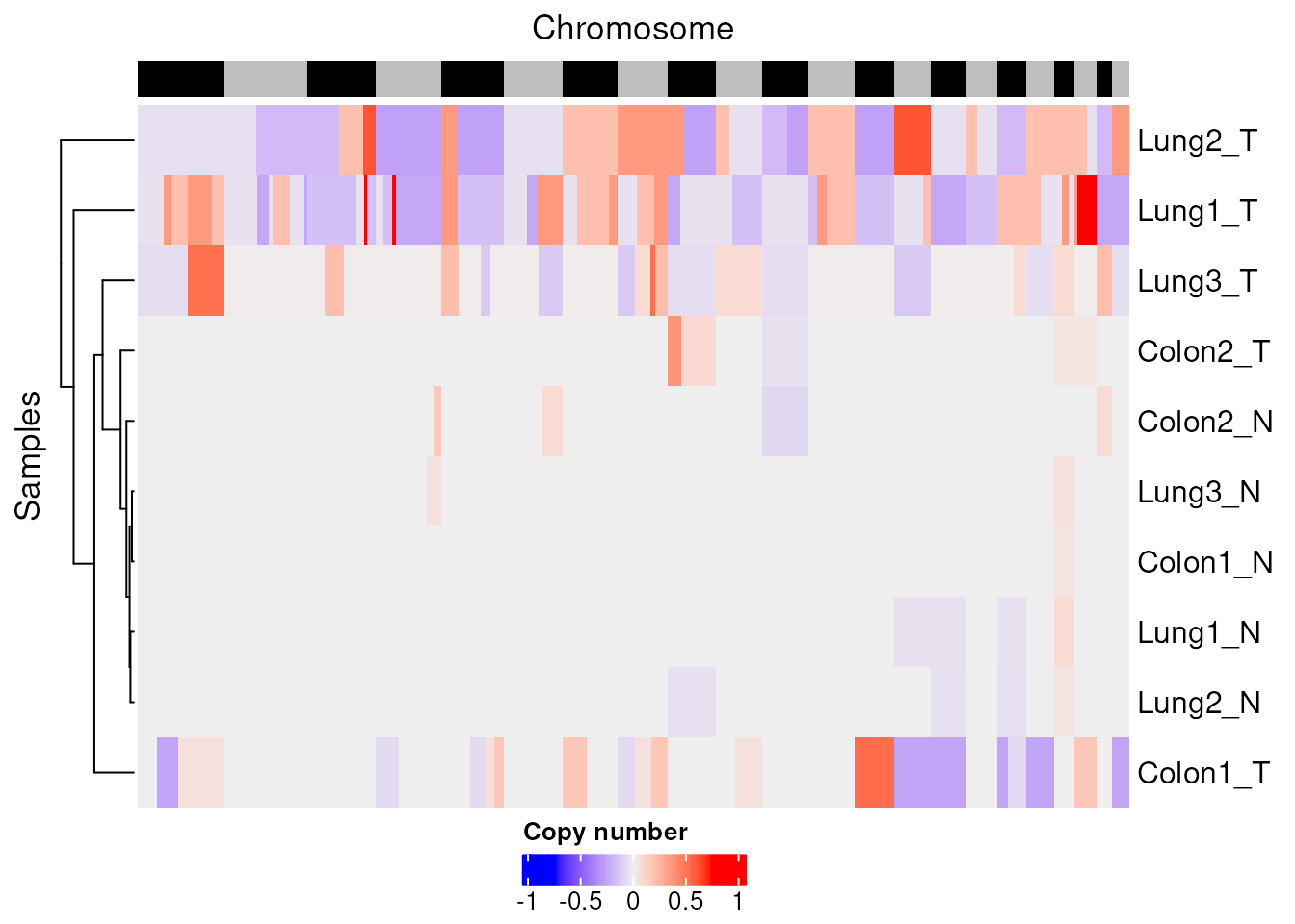
Parameters, Enrichment, Zygosity
There are also three other slots of the qseaSet, where it stores
internal information: parameters, a list of the parameters
that were used to generate the qseaSet; enrichment, the
fitted enrichment parameters used to calculate beta values; and
zygosity, the expected number of copies of each chromosome
in each sample.
These should not typically need to be modified or accessed.
Parallelisation
Finally, we will mention how parallelisation within the
mesa functions is set up. The functions inside the package
use the BiocParallel package, and will automatically check
if parallelisation has been turned on. This is controlled via the global
option value of mesa_parallel:
options("mesa_parallel")
#> $mesa_parallel
#> NULL
To set this, we use the setMesaParallel function:
setMesaParallel(useParallel = TRUE, nCores = 2)
#> Parallelisation turned on for the functions in the mesa package, currently using 2 cores.
#> Control the number of cores by calling BiocParallel::register.
The use of nCores here will set up a
MulticoreParam architecture with that many cores (a
reasonable default for Linux or macOS). Specify a different architecture
with BiocParallel::register if you wish to vary this; see
the BiocParallel vignette for how to specify one,
vignette("Introduction_To_BiocParallel", package = "BiocParallel").
The most recently registered instance will be used.
Setting this parameter globally via options means that
we don’t have to explicitly pass parallel = TRUE to
functions in order for them to parallelise across the available
cores.
Session info
#> R version 4.6.1 (2026-06-24)
#> Platform: x86_64-pc-linux-gnu
#> Running under: Ubuntu 24.04.4 LTS
#>
#> Matrix products: default
#> BLAS:   /usr/lib/x86_64-linux-gnu/openblas-pthread/libblas.so.3
#> LAPACK: /usr/lib/x86_64-linux-gnu/openblas-pthread/libopenblasp-r0.3.26.so;  LAPACK version 3.12.0
#>
#> locale:
#>  [1] LC_CTYPE=en_US.UTF-8       LC_NUMERIC=C
#>  [3] LC_TIME=en_US.UTF-8        LC_COLLATE=en_US.UTF-8
#>  [5] LC_MONETARY=en_US.UTF-8    LC_MESSAGES=en_US.UTF-8
#>  [7] LC_PAPER=en_US.UTF-8       LC_NAME=C
#>  [9] LC_ADDRESS=C               LC_TELEPHONE=C
#> [11] LC_MEASUREMENT=en_US.UTF-8 LC_IDENTIFICATION=C
#>
#> time zone: UTC
#> tzcode source: system (glibc)
#>
#> attached base packages:
#> [1] stats     graphics  grDevices utils     datasets  methods   base
#>
#> other attached packages:
#> [1] mesa_0.99.8.9000 dplyr_1.2.1      qsea_1.38.0
#>
#> loaded via a namespace (and not attached):
#>  [1] tidyselect_1.2.1            Biostrings_2.80.2
#>  [3] bitops_1.1-0                fastmap_1.2.0
#>  [5] RCurl_1.98-1.20             GenomicAlignments_1.48.0
#>  [7] XML_3.99-0.25               digest_0.6.39
#>  [9] lifecycle_1.0.5             cluster_2.1.8.3
#> [11] plyranges_1.32.0            statmod_1.5.2
#> [13] magrittr_2.0.5              compiler_4.6.1
#> [15] rlang_1.3.0                 sass_0.4.10
#> [17] tools_4.6.1                 utf8_1.2.6
#> [19] yaml_2.3.12                 data.table_1.18.6.1
#> [21] rtracklayer_1.72.0          knitr_1.52
#> [23] S4Arrays_1.12.1             htmlwidgets_1.6.4
#> [25] curl_8.1.0                  DelayedArray_0.38.2
#> [27] RColorBrewer_1.1-3          abind_1.4-8
#> [29] BiocParallel_1.46.0         HMMcopy_1.54.0
#> [31] withr_3.0.3                 purrr_1.2.2
#> [33] BiocGenerics_0.58.1         desc_1.4.3
#> [35] grid_4.6.1                  stats4_4.6.1
#> [37] colorspace_2.1-4            iterators_1.0.14
#> [39] gtools_3.9.5                SummarizedExperiment_1.42.0
#> [41] cli_3.6.6                   rmarkdown_2.32
#> [43] crayon_1.5.3                ragg_1.5.2
#> [45] generics_0.1.4              otel_0.2.0
#> [47] httr_1.4.9                  rjson_0.2.23
#> [49] cachem_1.1.0                stringr_1.6.0
#> [51] parallel_4.6.1              XVector_0.52.0
#> [53] restfulr_0.0.17             matrixStats_1.5.0
#> [55] vctrs_0.7.3                 Matrix_1.7-6
#> [57] jsonlite_2.0.0              GetoptLong_1.1.1
#> [59] IRanges_2.46.0              S4Vectors_0.50.3
#> [61] clue_0.3-68                 systemfonts_1.3.2
#> [63] foreach_1.5.2               limma_3.68.5
#> [65] jquerylib_0.1.4             glue_1.8.1
#> [67] pkgdown_2.2.1               codetools_0.2-20
#> [69] shape_1.4.6.1               stringi_1.8.9
#> [71] GenomeInfoDb_1.48.0         BiocIO_1.22.0
#> [73] GenomicRanges_1.64.0        UCSC.utils_1.8.0
#> [75] ComplexHeatmap_2.28.0       tibble_3.3.1
#> [77] pillar_1.11.1               htmltools_0.5.9
#> [79] Seqinfo_1.2.0               circlize_0.4.18
#> [81] BSgenome_1.80.0             R6_2.6.1
#> [83] textshaping_1.0.5           doParallel_1.0.17
#> [85] evaluate_1.0.5              lattice_0.23-1
#> [87] Biobase_2.72.0              png_0.1-9
#> [89] Rsamtools_2.28.0            cigarillo_1.2.1
#> [91] memoise_2.0.1               bslib_0.12.0
#> [93] SparseArray_1.12.3          xfun_0.61
#> [95] GlobalOptions_0.1.4         fs_2.1.0
#> [97] MatrixGenerics_1.24.0       zoo_1.9-1
#> [99] pkgconfig_2.0.3