Distribution of windows across genomic features
Source:R/plotting.R
plotGenomicFeatureDistribution.RdAnnotate windows (e.g., promoters/exons/introns) and plot the distribution per sample as stacked/dodged/filled bars.
plotGenomicFeatureDistribution(
  qseaSet,
  cutoff = 1,
  barType = "stack",
  normMethod = "nrpm",
  genome = NULL,
  TxDb = NULL,
  annoDb = NULL
)
Arguments
- qseaSet
qseaSet. Input object containing windows and signal (beta or nrpm).- cutoff
numeric(1). Threshold applied to the chosen normalisation measure per window. Default:1.- barType
character(1). Bar layout: one of"stack","dodge", or"fill"(relative proportions). Default:"stack".- normMethod
character(1). Normalisation/measure to threshold. One of"nrpm"or"beta". Default:"nrpm".- genome
character(1)orNULL. Genome build (e.g.,"hg38","hg19","mm10"). If provided, uses mesa's genome system viagetMesaTxDb()andgetMesaAnnoDb(). Default:NULL(usesTxDbandannoDbparameters).- TxDb
TxDbobject orNULL. Transcript database for gene annotation. Ignored ifgenomeis provided. Default:TxDb.Hsapiens.UCSC.hg38.knownGenefor backward compatibility.- annoDb
character(1)orNULL. Annotation database name (e.g.,"org.Hs.eg.db"). Ignored ifgenomeis provided. Default:"org.Hs.eg.db".
Value
A ggplot2 object showing counts (or proportions, for "fill")
of feature classes per sample above cutoff.
Details
Feature classes are taken from region annotations available on the windows
(e.g., columns produced by annotateWindows() such as
shortAnno/annotation,
if present). Bars are positioned according to barType
(stack/dodge/fill).
See also
annotateWindows(), qsea::makeTable(), ggplot2::geom_bar()
Other annotation-summaries:
getGenomicFeatureDistribution()
Examples
# Recommended workflow: set genome globally (saving the current setting)
oldGenome <- getOption("mesa_genome")
setMesaGenome("hg38")
data(exampleTumourNormal, package = "mesa")
# Uses global hg38 setting
if (requireNamespace("TxDb.Hsapiens.UCSC.hg38.knownGene", quietly = TRUE) &&
requireNamespace("org.Hs.eg.db", quietly = TRUE)) {
exampleTumourNormal %>%
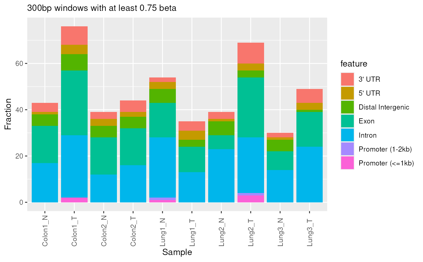
plotGenomicFeatureDistribution(normMethod = "beta", cutoff = 0.75)
}
#> obtaining raw values for 10 samples in 819 windows
#> deriving beta values...
#> creating table...
#> >> Using Genome: hg38 ...
#> >> Using Genome: hg38 ...
#> >> Using Genome: hg38 ...
#> 'select()' returned 1:1 mapping between keys and columns
#> Don't know how to automatically pick scale for object of type <table>.
#> Defaulting to continuous.
#> Ignoring unknown labels:
#> • legend : "Feature"
 # \donttest{
# Override for specific analysis
exampleTumourNormal %>%
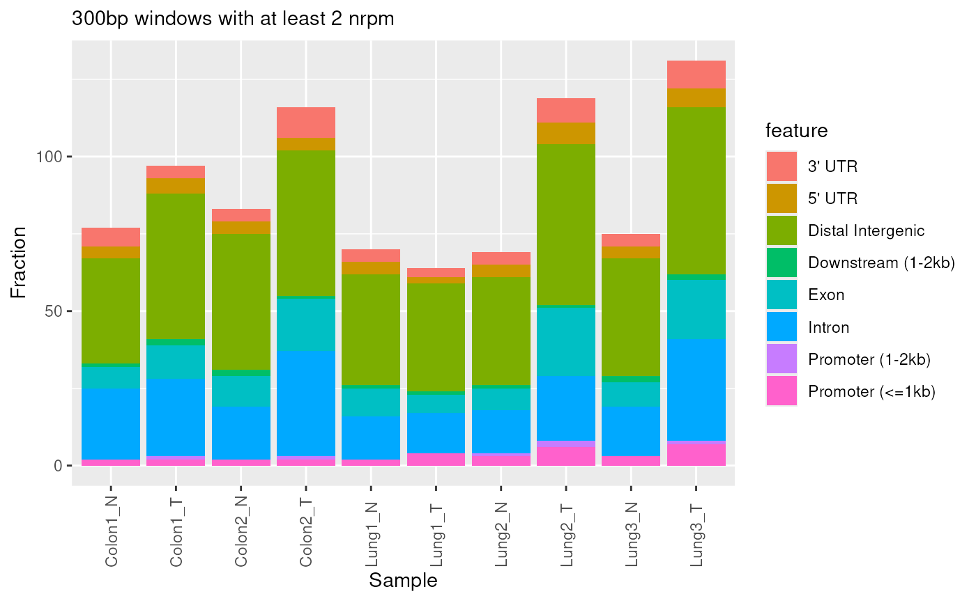
plotGenomicFeatureDistribution(
genome = "mm10",
normMethod = "nrpm",
cutoff = 2
)
#> obtaining raw values for 10 samples in 819 windows
#> deriving nrpm values...
#> creating table...
#> >> Update txdb in cache...
#> >> Using Genome: mm10 ...
#> >> Using Genome: mm10 ...
#> >> Using Genome: mm10 ...
#> 'select()' returned 1:1 mapping between keys and columns
#> Don't know how to automatically pick scale for object of type <table>.
#> Defaulting to continuous.
#> Ignoring unknown labels:
#> • legend : "Feature"
# \donttest{
# Override for specific analysis
exampleTumourNormal %>%
plotGenomicFeatureDistribution(
genome = "mm10",
normMethod = "nrpm",
cutoff = 2
)
#> obtaining raw values for 10 samples in 819 windows
#> deriving nrpm values...
#> creating table...
#> >> Update txdb in cache...
#> >> Using Genome: mm10 ...
#> >> Using Genome: mm10 ...
#> >> Using Genome: mm10 ...
#> 'select()' returned 1:1 mapping between keys and columns
#> Don't know how to automatically pick scale for object of type <table>.
#> Defaulting to continuous.
#> Ignoring unknown labels:
#> • legend : "Feature"
 # Advanced: manual control (bypasses mesa genome system)
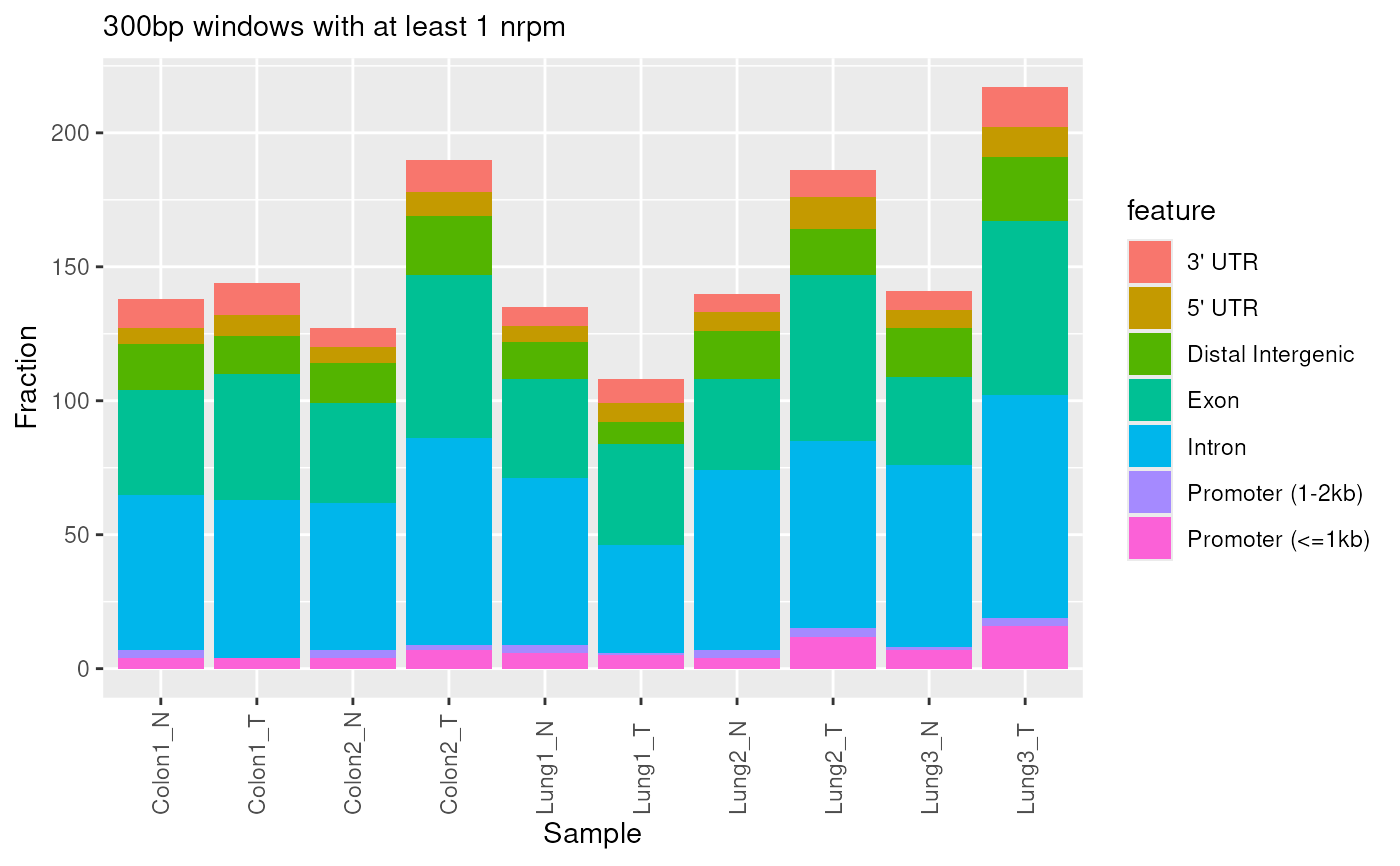
exampleTumourNormal %>%
plotGenomicFeatureDistribution(
TxDb = TxDb.Mmusculus.UCSC.mm10.knownGene::
TxDb.Mmusculus.UCSC.mm10.knownGene,
annoDb = "org.Mm.eg.db"
)
#> obtaining raw values for 10 samples in 819 windows
#> deriving nrpm values...
#> creating table...
#> >> Update txdb in cache...
#> >> Using Genome: hg38 ...
#> >> Using Genome: hg38 ...
#> >> Using Genome: hg38 ...
#> 'select()' returned 1:1 mapping between keys and columns
#> Don't know how to automatically pick scale for object of type <table>.
#> Defaulting to continuous.
#> Ignoring unknown labels:
#> • legend : "Feature"
# Advanced: manual control (bypasses mesa genome system)
exampleTumourNormal %>%
plotGenomicFeatureDistribution(
TxDb = TxDb.Mmusculus.UCSC.mm10.knownGene::
TxDb.Mmusculus.UCSC.mm10.knownGene,
annoDb = "org.Mm.eg.db"
)
#> obtaining raw values for 10 samples in 819 windows
#> deriving nrpm values...
#> creating table...
#> >> Update txdb in cache...
#> >> Using Genome: hg38 ...
#> >> Using Genome: hg38 ...
#> >> Using Genome: hg38 ...
#> 'select()' returned 1:1 mapping between keys and columns
#> Don't know how to automatically pick scale for object of type <table>.
#> Defaulting to continuous.
#> Ignoring unknown labels:
#> • legend : "Feature"
 # }
# Restore the previous genome setting
options(mesa_genome = oldGenome)
# }
# Restore the previous genome setting
options(mesa_genome = oldGenome)