Generate publication-ready plots from the output of getPCA(). The function
supports flexible visual encodings (colour, shape, size) of sample-level
metadata and can return multiple plots across different PC pairs and
annotation variables.
Arguments
- object
mesaDimRed. A dimensionality-reduction container returned bygetPCA().- components
integer(2)orlistofinteger(2). PC indices to plot (e.g.c(1, 2)for PC1 vs PC2), or a list of such pairs to produce multiple plots. Default:list(c(1, 2), c(2, 3)).- colour
NULLorcharacter(). Name(s) of sample-table variable(s) mapped to point colour; one plot per variable. Default:NULL(no colour mapping).- colourPalette
NULLorcharacter(). Palette used for colouring points. IfNULL, a suitable default is chosen. Default:NULL.- NAcolour
character(1). Colour for missing values incolour. Default:"grey50".- symDivColourScale
logical(1). IfTRUE, diverging colour scales are centred symmetrically around zero. Ignored for non-diverging scales. Default:FALSE.- shape
NULLorcharacter(1). Sample-table variable mapped to point shape (single variable only). Default:NULL.- shapePalette
NULL,character(1), ornumeric(). Shapes used for categories of theshapevariable. Options:A numeric vector of base‐R shape codes.
0–20: line/filled shapes.
21–25: filled shapes with a border (border colour = black).
A keyword, with internally defined sets:
"line-first": 15 line shapes, then 4 filled shapes (max 19 categories)."filled-first": 4 filled shapes, then 15 line shapes (max 19 categories)."mixture": mixture of line and filled shapes (max 19 categories).
"filled+border": filled+border shapes (max 5 categories, or 4 if NAs inshape).
NULL: choose automatically ("mixture"for non-diverging/none;"filled+border"for diverging colour scales). Default:NULL.
- NAshape
NULLornumeric(1). Shape for missing values inshape. IfNULL, uses7, or25when"filled+border"is active. Default:NULL.- showSampleNames
logical(1). Overlay sample names on points. Default:FALSE.- pointSize
numeric(1). Point size. Default:2.- alpha
numeric(1). Point transparency in[0, 1]. Default:1.- plotlyAnnotations
character(). Column names from the sample table to add as tooltips when converting to interactiveplotly. Default:""(empty string).
Value
A list of ggplot objects—one per combination of components
pairs and colour variables—each depicting the chosen PCs with requested
aesthetics. Specifically:
one plot per
componentspair × percolourvariable;shapes/labels applied per
shape/showSampleNames;consistent axis labelling (PC variance if available).
Details
Shape defaults
"mixture"is used for non-diverging or discrete colour scales (or no colour)."filled+border"is used for diverging colour scales. These defaults aim to keep categories visually separable for larger cohorts.
See also
Examples
data(exampleTumourNormal, package = "mesa")
# Basic PCA plot (PC1 vs PC2) with defaults
exampleTumourNormal %>%
getPCA() %>%
plotPCA()
#> ------------------------------
#> Initial number of windows = 819.
#> -----------
#> Generating table of beta values for 819 regions across 10 samples.
#> -----------
#> Filtered out 220 windows with at least one missing value: 599 windows remaining.
#> ------------------------------
#> The following topVarNum values are larger than the number of remaining windows (= 599): 1000
#> These values are not used; PCA will be done with all remaining windows instead.
#> ------------------------------
#> No filtering of windows based on window standard deviation.
#> Performing PCA with 10 samples and 599 windows
#> -> pca1.
#> ------------------------------
#> $pca1
#> $pca1$PC1vsPC2
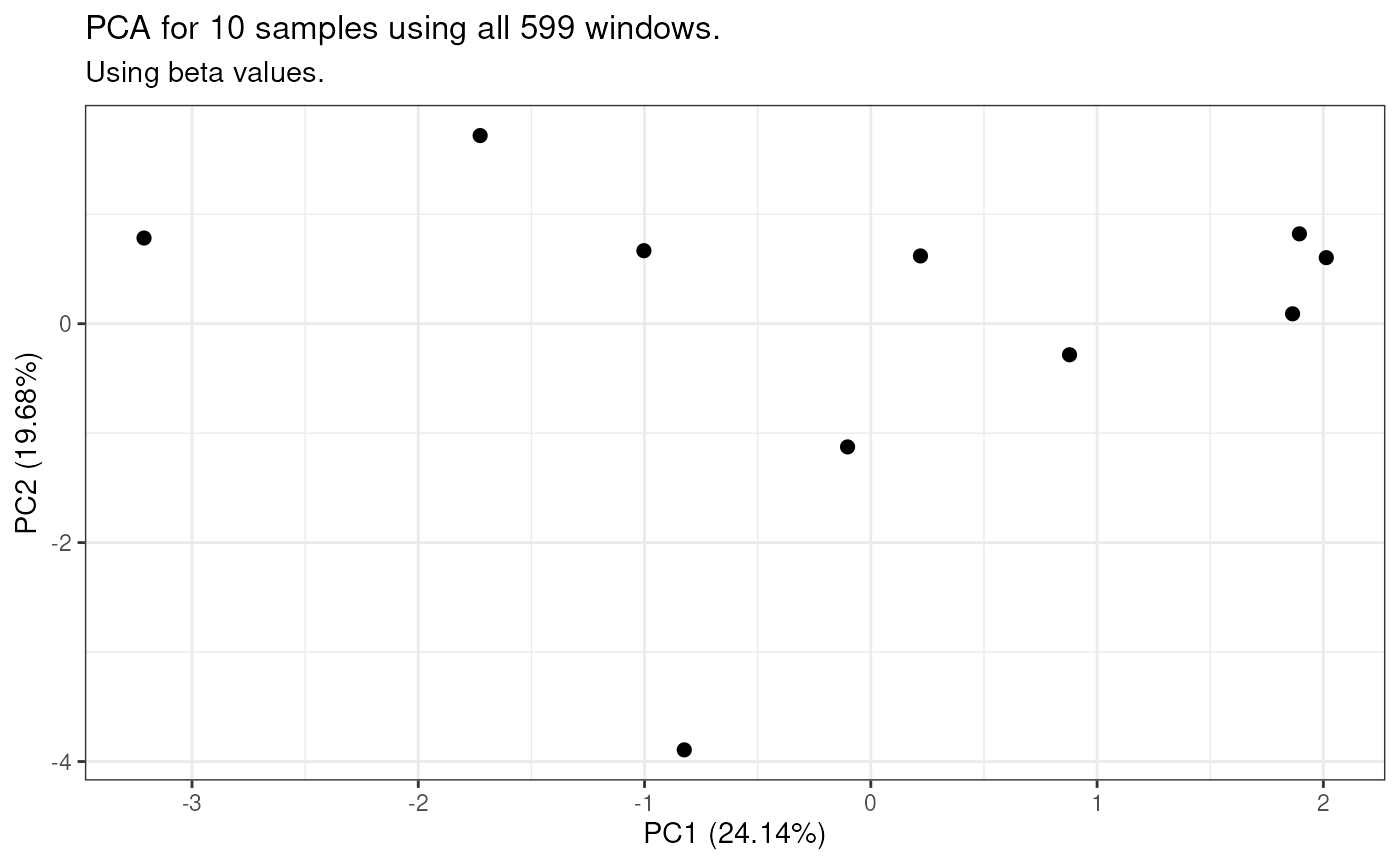 #>
#> $pca1$PC2vsPC3
#>
#> $pca1$PC2vsPC3
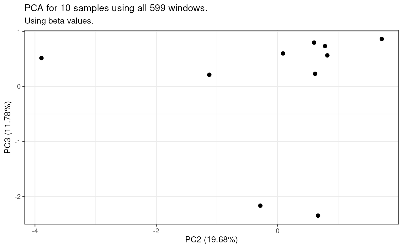 #>
#>
# Colour by sample group; show names
exampleTumourNormal %>%
getPCA() %>%
plotPCA(
colour = "group",
showSampleNames = TRUE
)
#> ------------------------------
#> Initial number of windows = 819.
#> -----------
#> Generating table of beta values for 819 regions across 10 samples.
#> -----------
#> Filtered out 220 windows with at least one missing value: 599 windows remaining.
#> ------------------------------
#> The following topVarNum values are larger than the number of remaining windows (= 599): 1000
#> These values are not used; PCA will be done with all remaining windows instead.
#> ------------------------------
#> No filtering of windows based on window standard deviation.
#> Performing PCA with 10 samples and 599 windows
#> -> pca1.
#> ------------------------------
#> $pca1
#> $pca1$group
#> $pca1$group$PC1vsPC2
#>
#>
# Colour by sample group; show names
exampleTumourNormal %>%
getPCA() %>%
plotPCA(
colour = "group",
showSampleNames = TRUE
)
#> ------------------------------
#> Initial number of windows = 819.
#> -----------
#> Generating table of beta values for 819 regions across 10 samples.
#> -----------
#> Filtered out 220 windows with at least one missing value: 599 windows remaining.
#> ------------------------------
#> The following topVarNum values are larger than the number of remaining windows (= 599): 1000
#> These values are not used; PCA will be done with all remaining windows instead.
#> ------------------------------
#> No filtering of windows based on window standard deviation.
#> Performing PCA with 10 samples and 599 windows
#> -> pca1.
#> ------------------------------
#> $pca1
#> $pca1$group
#> $pca1$group$PC1vsPC2
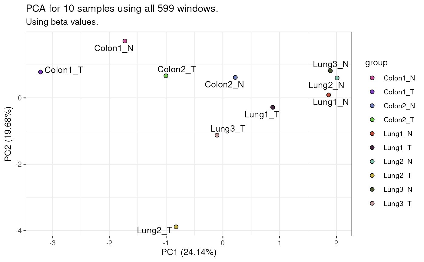 #>
#> $pca1$group$PC2vsPC3
#>
#> $pca1$group$PC2vsPC3
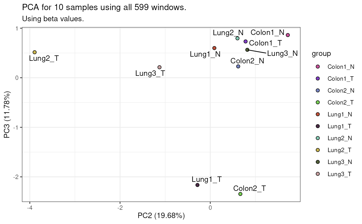 #>
#>
#>
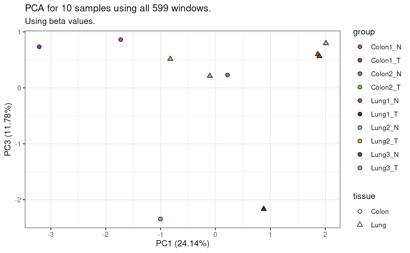
# Plot PC1 vs PC3; shape by tissue
exampleTumourNormal %>%
getPCA() %>%
plotPCA(
components = list(c(1, 3)),
colour = "group",
shape = "tissue"
)
#> ------------------------------
#> Initial number of windows = 819.
#> -----------
#> Generating table of beta values for 819 regions across 10 samples.
#> -----------
#> Filtered out 220 windows with at least one missing value: 599 windows remaining.
#> ------------------------------
#> The following topVarNum values are larger than the number of remaining windows (= 599): 1000
#> These values are not used; PCA will be done with all remaining windows instead.
#> ------------------------------
#> No filtering of windows based on window standard deviation.
#> Performing PCA with 10 samples and 599 windows
#> -> pca1.
#> ------------------------------
#> $pca1
#> $pca1$group
#> $pca1$group$PC1vsPC3
#>
#>
#>
# Plot PC1 vs PC3; shape by tissue
exampleTumourNormal %>%
getPCA() %>%
plotPCA(
components = list(c(1, 3)),
colour = "group",
shape = "tissue"
)
#> ------------------------------
#> Initial number of windows = 819.
#> -----------
#> Generating table of beta values for 819 regions across 10 samples.
#> -----------
#> Filtered out 220 windows with at least one missing value: 599 windows remaining.
#> ------------------------------
#> The following topVarNum values are larger than the number of remaining windows (= 599): 1000
#> These values are not used; PCA will be done with all remaining windows instead.
#> ------------------------------
#> No filtering of windows based on window standard deviation.
#> Performing PCA with 10 samples and 599 windows
#> -> pca1.
#> ------------------------------
#> $pca1
#> $pca1$group
#> $pca1$group$PC1vsPC3
 #>
#>
#>
#>
#>
#>